
This is what I have learned after writing the Azure AI fundamentals exam.
Overview
Artificial intelligence is the software that imitates human behaviours and capabilities. AI encompasses a very broad range of areas. In Azure’s product offering, it breaks it down into four application areas: Machine Learning, Computer Vision, Natural language processing and conversational AI. Note that the media, sometimes including tech companies, tend to use the terms AI and ML interchangeably, which is incorrect. ML did not really surface as a key driver of AI commercially, until the last 10 – 15 years. However, other areas of AI, such as computer vision and natural language processing had been around for a quite a while.

Now we know the distinction between AI and ML: ML is just one of the many areas of AI but it has recently become the most attention-grabbing and cutting-edge area. We will introduce ML the last.
Computer Vision
Computer Vision is the ability of software to interpret the world visually through cameras, video and images. It has the following application scenarios:
- Image Classification: training ML model to classify images based on contents.
- Object Detection: training ML model to classify individual objects within an image, and identify their location with bounding box.
- Semantic Segmentation: An advanced ML technique in which individual pixels in the image are classified according to the object to which they belong. This forms mask layer
- Image Analysis: extract information from images
- Face detection, analysis, and recognition: specialized form of object detection that locates human face in image. This can be combined with classification and facial geometry analysis techniques to infer details such as gender, age, and emotional state. Face detection is impaired by extreme angles.
- OCR: detect and read text in images.
The model training process is an iterative process in which the Custom Vision service repeatedly trains the model using some of the data, but holds some back to evaluate the model. The evaluation metrics include:
- precision: what percentage of the class predictions made by the model were correct. E.g. model predicts 10 images are oranges. 8 actually are. Precision = 0.8
- recall: what percentage of class predictions did the model correctly identify. E.g. 10 images of apples, the model find 7. recall = 0.7
- AP (average precision): an overall metric that takes into account both precision and recall.
Azure-specific: in Azure, computer vision services include:
- Computer Vision: analyze images and video, and extract descriptions, tags, objects and text;
- Custom Vision: train custom image classification (two special form: celebrity and landscape) and object detection models using your own image;
- Face: build face detection and facial recognition solutions
- Form recognizer: extract information from scanned forms and invoices
Azure-specific: difference between Computer Vision and Cognitive Service
- Computer Vision: A specific resource for the computer vision services. Use this type of resource if you don’t intend to use any other cognitive services. Or if you want to track utilization and costs for your computer vision resource separately
- Cognitive Service: A general cognitive service resource that include Computer Vision along with many other cognitive services, such as Text Analytics, Translator Text, and others. Use this resource type if you plan to use multiple cognitive services and want to simplify administration and development.
Natural Language Processing
NLP is the ability of computer to interpret written or spoken language, and respond in kind.
- Analyze text
- Recognize (speech-to-text api) and synthesize speech (text-to-speech api to generate spoken output)
- Translate text and speech
- Language understanding
Models that you use to accomplish speech recognition:
- acoustic model – converts audio signal into phonemes (representations of specific sounds)
- language model – maps phonemes to words, usually using a statistical algorithm that predicts the most probable sequence of words based on the phonemes
Core concepts in language understanding
- utterance – an example of something a user might say, and your application must interpret. Eg. Switch the fan on. Turn on the light.
- entities – an item to which an utterance refers. e.g. fan, light. four types of entities: machine-learned, list, regex, pattern.any
- intents – represents the purpose, or goal, expressed in user’s utterance. E.g. Turn on
- None intent
Azure-specific: To create a language understanding application:
- First you must define entities, intents, and utterances with which to train the language model — referred to as authoring the model
- Then you must publish the model so that client applications can use it for intent and entity prediction based on user input
Azure-specific: in Azure, NLP services include
- Text Analytics: analyze text documents and extract key phrases, detect entities (places, people, dates), and evaluate sentiment (positive, negative). mixed language or ambiguous content will produce “NaN” in the result.
- Translator Text: translate text between languages
- Speech: recognize and synthesize speech, and translate spoken language
- Language Understanding Intelligent Service (LUIS): train a language model that can understand spoken or text-based commands.
Conversational AI
This is the capability of a software agent to participate in a conversation.
Azure-specific: Azure Bot service is a platform for creating, publishing and managing bots. Developers can use the Bot Framework to create a bot and manage it with Azure Bot service – integrating back-end services like QnA maker and LUIS, and connecting to channels for web chat. QnA Maker enables you to quickly build a knowledge base of questions and answers that can form the basis of a dialog between a human and an AI agent.
Machine Learning
The reason I put machine learning the last, is because it’s most important, and it involves some brain-burning mathematical details. Machine learning is a technique that uses mathematics and statistics to create a model that can predict unknown values. Machine learning is based on huge volumes of data. Data scientist can use all of that data to train machine learning models that can make predictions and inferences based on the relationships they find in the data.

There are so many sub-areas of machine learning and Google has an entire crash course for it. As far as application is concerned, we need to first match a new problem with an existing problem, and from there pick an appropriate algorithm. There is a cheat sheet for such purpose for Azure services. For learning purpose, we should focus on three problems. Before getting to that, we need to first distinguish supervised learning and unsupervised learning:
- Supervised learning: you train the machine using data which is well “labelled”. So some data is already tagged with correct answer. A supervised learning algorithm learns from labelled training data, and helps you predict outcomes for unforeseen data. Two typical types of supervised learning techniques are classification, and regression.
- Unsupervised learning: you do not need to supervise the model. Instead, you need to allow the model to work on its own to discover information by dealing with unlabeled data. Typical unsupervised learning technique is clustering. It mainly deals with finding a structure or pattern in a collection of uncategorized data.
So the three problem we are going to focus on are:
- Regression Model (supervised): Use historic data to train the model to predict the numerical value
- Classification Model (supervised): fit the features into the model and predict the classification of the label
- Clustering Model (unsupervised): you don’t have a label to predict. you only have features. You have to group similar items into clusters based on features.
Now we will review how to assess the learning model in each technique:
Performance Metrics for Regression Model
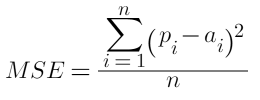
In all of the equations below, pi denotes predicted value, ai denotes actual value, and ā denotes the mean of actual values.
- Mean Absolute Error (MAE):
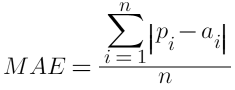
- It has the same unit with original data so it only can be used to compare models whose errors are measured in the same unit.
- It has similar magnitude as RMSE (as will discuss below), but smaller in value
- The lower this value is, the better the model is predicting.
2. Mean Square Error (MSE):
3. Root Mean Square Error (RMSE):
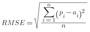
- It measures the error rate of a regression model
- It can only be compared between models whos errors are measured in the same unit.
- RMSE and SD (standard deviation) have similar (not same) formula yet different purposes. SD measures the spread of data around the mean. RMSE measures the error of prediction (predicted vs true). The two formula produce the same result only if you use the mean as prediction.
4. Relative Square Error (RSE):
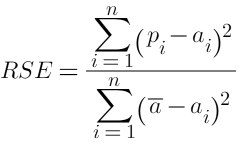
- A relative metric between 0 and 1. It has no units so can be used to compare models whose errors are measured in different units.
- The closer to 0 this metric is, the better the model is performing
5. Relative Absolute Error (RAE):
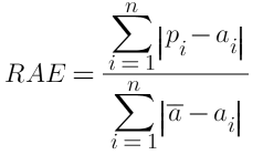
- A relative metric between 0 and 1. It has no units so can be used to compare models whose errors are measured in different units.
- The closer to 0 this metric is, the better the model is performing
6. Coefficient of determination (R2):
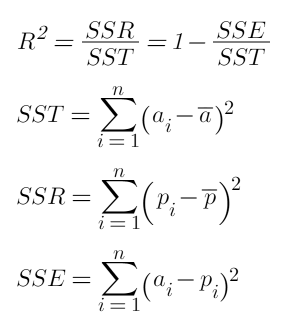
- Also known as r-squared. It summarizes the explanatory power of the regression model. In other words, how much of the variance between predicted and actual values is explained by the model.
- It is computed from the sums-of-squares terms, including Sum of Squares Total (SST), Sum of Squares Regression (SSR), and Sum of Squares Error (SSE), as illustrated above.
- R2 describes the proportion of variance of the dependent variable explained by the regression model
- The closer to 1 this value is, the better the model is performing. If the regression model is perfect, SSE = 0, R2 = 1
- If the regression is a total failure, SSE=SST, no variance is explained by regression, and R2 = 0
Performance Metrics for Classification Model
Now we review the metrics for classification model. Credit to this positing. Let’s go start with some classification result, more famously known as confusion matrix:
| classified as negative | classified as positive | ||
| actually negative | TN=9000 | FP=700 | 9700 are actually negative (TN+FP) |
| actually positive | FN=200 | TP=100 | 300 are actually positive (FN+TP) |
| 9100 classified correctly (TN+TP) | 900 classified incorrectly (FN+FP) |
Note that what a classification model predicts is the probability for each possible class. In the case of binary classification model, we can set a threshold (e.g. 0.5), such that predictions greater than 0.5 indicates positive, otherwise negative. So for each classification result, a changing threshold would change each value in the quadrant.
- Accuracy:
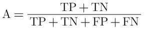
- The ratio of correct predictions (true) to the total number of predictions.
- Indicates out of all the predictions, how much are identified correctly by the model
- This metric is intuitive but not very useful (e.g. 3% of population is diabetic, then a model that always predicts false would be 97% accurate…) so data scientists use other metrics like precision and recall to assess classification model performance
2. Precision:
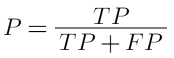
- The fraction of positive cases correctly identified.
- Indicates out of all the positive predictions, how much are actually true case.
- In other words, in your catch, what percent are actually a problem.
- This is much more useful than accuracy. Example: out of all the cases identified as diabetics, the rate of correct identifications.
3. Recall:
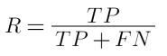
- The fraction of the cases classified as positive that are actually positive
- Indicates out of all the positive cases, how much are identified by the model
- Also known as true positive rate (TPR); and is also much more useful than accuracy. Example: out of all the real diabetics cases, the rate of the ones correctly identified by model.
- In other words, what percent of the problem did the model catch.
Going over the example data in the confusion matrix, Accuracy=0.91 , Precision=0.125, Recall=0.333 and now you see how useless accuracy is. The more uneven the class distribution is, the less useful accuracy is.
4. F1 score:
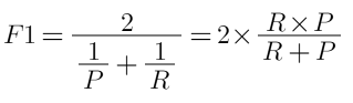
- F1 score combines Recall and Precision to one performance metrics with weighted average.
- So it takes both false positives (the problems the model caught wrong) and false negatives (the problems the model failed to catch) into account.
- F1 is useful because you always have to use both Recall and Precision.
5. In addition, there is a metric called FPR (false positive rate) in compliment to TPR (recall):
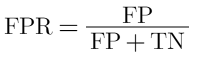
- It indicates what percent in the catch did the model get wrong.
We learned that both recall and precision needs to be looked at when assessing a classification model. Unfortunately, Precision and Recall are often in tension: improving one typically reduces the other. We’ve also learned that, those performance metrics are different as threshold changes.
6. ROC curve: to summarize performance over all possible thresholds, we introduce the ROC curve. The name ROC (Receiver Operating Characteristics) stems historically from communications theory. The ROC curve is created by plotting the TRP against the FPR, at different thresholds. It indicates how well your classification model can separate positive and negative examples and to identify the best threshold for separating them.

Below is the result of the ROC curve

7. AUC (Area Under the Curve)
The model performance is determined by looking at the area under the ROC curve (aka AUC), which can range from 0 to 1. The larger the AUC, the better the model is performing. An excellent model has AUC near 1.0, indicating a great ability to separate positive from negative, as opposed to random guessing (coin flipping):

That’s it for classification…
Performance Metrics for Clustering Model
Evaluating a clustering model is difficult by the fact that there are no previously known true values for the cluster assignments. A successful clustering model is defined as one that achieves a good level of separation between the items in each cluster, so we need metrics to help us measure that separation.
A common clustering algorithm is K-Means Clustering. Below are some measurements:
- Average Distance to Other Centre: indicates how close, on average, each point in the cluster is to the centroids of all other clusters.
- Average Distance to Cluster Centre: indicates how close, on average, each point in the cluster is to the centroid of the cluster.
- Number of Points: the number of points assigned to the cluster.
- Maximal Distance to Cluster Centre: the maximum of the distances between each point and the centroid of that point’s cluster. If this number is high, the cluster may be widely dispersed. This statistic in combination with the Average Distance to Cluster Center helps you determine the cluster’s spread.
Azure-specific: Azure Machine Learning service provides cloud-based platform for creating, managing and publishing machine learning models. including:
- automated machine learning
- Azure machine learning designer (no-code development environment)
- Data and computer management
- Pipelines: to orchestrate model training, deployment and manage tasks.
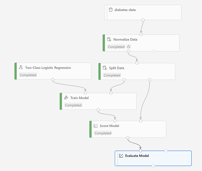
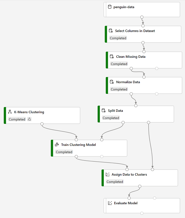
Here’s what pipelines typically look like:
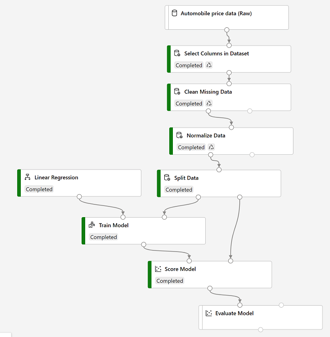
Machine Learning studio (ml.azure.com) provides a more focused UI for managing workspace resources. The following kinds of compute resources can be used to train models:
- compute instances: development workstation that data scientist can use to work with data and models
- compute clusters: scalable cluster of VMs for on-demand processing of experiment code
- inference clusters: deployment targets for predictive services that use your trained models
- attached computer: links to existing azure compute resources, such as VMs or data-bricks clusters